What is Sorting and Different Types of Sorting Algorithms
As an applied science engineering student one every of the foremost vital topics in algorithms on behalf of me is ‘Sorting’. So in this blog, we will discuss some important sorting algorithms.
SORTING ALGORITHM DEFINITION
Sorting refers to the operation of arranging the data given in some sequence in ascending or descending order.
IMPORTANCE OF SORTING
So why are sorting algorithms so important in our life? Putting data into ascending or descending order can be difficult and burdensome. Also, it makes our life easier to put things systematically around us. Well, we don’t even realize but we use sorting in our day-to-day life.
- Arranging clothes in the almirah
- Arranging books and files in a bookshelf
- Arranging utensils in kitchen cabinets
- Words in a dictionary
Sorting makes it easier for you to search for data. There are many sorting algorithms for different types of data.
- You arrange books according to the genre of the book
- You arrange utensils according to their shapes and size
- Words in the dictionary are arranged alphabetically
Example for sorting algorithm
Following are the examples of sorting algorithms:
- num=[1,5,8,78,45,3] ; num_sort=[1,3,5,8,45,78]
- alphabet=[b, g, j, l, k, m, r, h] ; alphabet_sort=[b, g, h, j, k, l, m, r]
- num1=[23,78,90,45,68] ; num1_sort=[23,45,68,78,90]
Types of sorting algorithms
There are many sorting algorithms like:
- Bubble Sort Algorithm
- Selection Sort Algorithm
- Quick Sort Algorithm
- Bubble Sort Algorithm
- Insertion Sort Algorithm
- Heap Sort Algorithm
- Merge Sort Algorithm
In this blog, we will discuss in detail these sorting algorithms.
SELECTION SORT
This algorithm sorts the array by continually searching the smallest element (ascending order) or maximum element (descending order) from the unsorted part of the array and putting it in the starting of the array. The algorithm maintains two subarrays: sorted and unsorted. In every iteration, the minimum element from the array is picked and fixed in the sorted array accordingly.
- Worst Case Time Complexity: O(n2)
- Best Case Time Complexity: O(n2)
- Average Time Complexity: O(n2)
- Space Complexity: O(1)
BUBBLE SORT
Sorting takes place by comparing all the elements one by one with the adjacent element and then swapping them if required. It will begin by comparison of the element selected with its successor element, if the second element is smaller than the first element then it swaps the two elements and then moves on to compare the second and the third element, and consequently. If we have n elements given in the array then the loop runs for n-1 times.
- Worst Case Time Complexity: O(n2)
- Best Case Time Complexity: O(n)
- Average Time Complexity: O(n2)
- Space Complexity: O(1)
INSERTION SORT
The array given as an input is split into a sorted and unsorted array, elements from the unsorted array are picked and placed at the correct position in the sorted part. To sort the array in descending order. iterate the array from arr[1] to arr[n]. Then compare the element chosen to its predecessor(previous element). And if the element is greater than its precursor, equate it to the elements given prior in the array. Move the smaller elements one position up to insert the swapped element.
- Worst Case Time Complexity: O(n2)
- Best Case Time Complexity: O(n)
- Average Time Complexity: O(n2)
- Space Complexity: O(1)
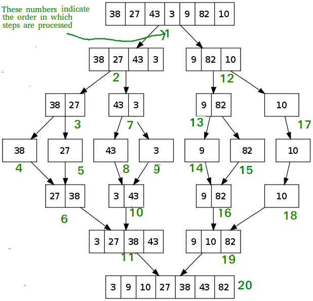
MERGE SORT
This sorting algorithm follows the DIVIDE AND CONQUER algorithm to sort the given data set. Here the data set is divided into multiple small data sets. Each data set is sorted individually and then finally all the sub-datasets are combined/merged to form the final sorted array.
Divide
If c is the mid/central point in the array between a and b, then we can split the subarray arr[a..b] into arr[a..c] and arr[c+1, r].
Conquer
In this step we sort both the subarrays: arr[a..c] and arr[c+1, r]. And if we haven’t reached the base case we divide both of them again and try to sort.
Combine
When we reach this step we have sorted subarrays and we combine the results of the previous step to form a sorted array.
- Best Case Complexity: O(n*log n)
- Worst Case Complexity: O(n*log n)
- Average Case Complexity: O(n*log n)
- Space Complexity: O(n).
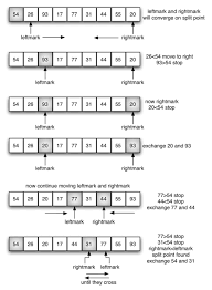
QUICK SORT Or PARTITION EXCHANGE SORT
Quicksort is a sorting algorithm based on the concept of DIVIDE AND CONQUER almost similar to merge sort. The algorithm starts by picking the element given in the data set as a pivot element and then divides the given array around the pivot. There are numerous methods to select pivot element such as:
- Picks the first element as pivot
- Picks the last element as pivot
- Picks a random element as pivot
- Picks median of the array as pivot
The algorithm is divided into three parts: Elements larger than pivot element, pivot element(mid element), and elements smaller than the pivot element. Firstly, the pivot will be set with elements smaller than the pivot to the left side of array and the elements larger than the pivot to the right of the array. Now the elements smaller and larger than the pivot element are considered as separate subarrays and recursive logic to sort the subarrays.
- Worst Case Time Complexity: O(n2)
- Best Case Time Complexity: O(n*log n)
- Average Time Complexity: O(n*log n)
- Space Complexity: O(n*log n)
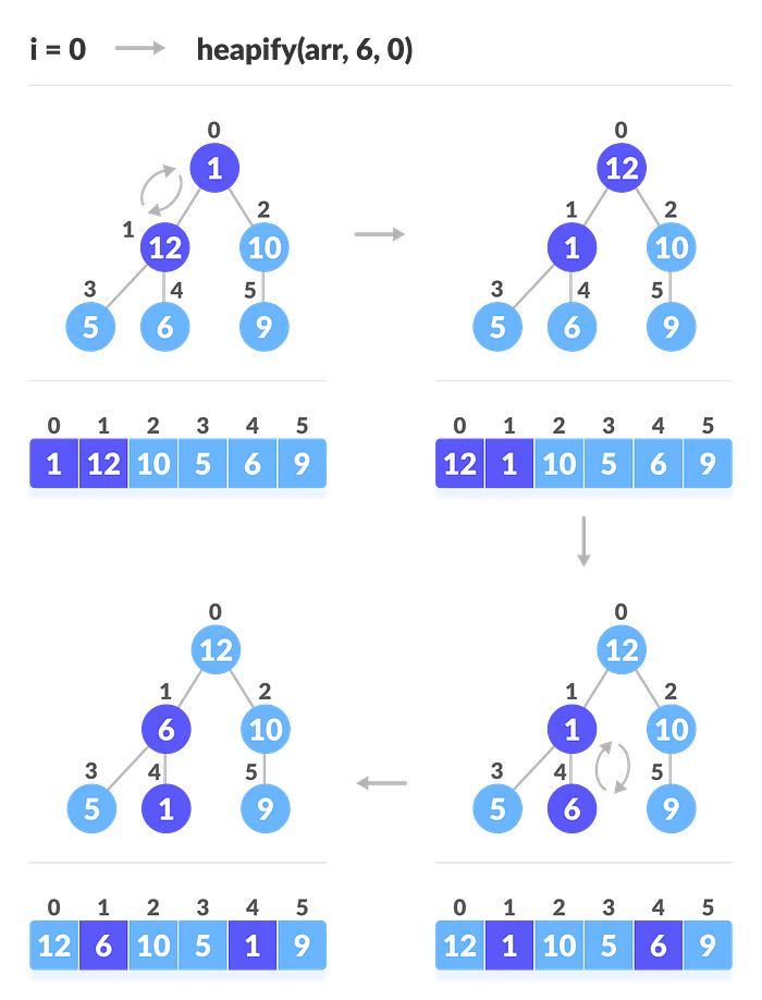
HEAP SORT
Heapsort is one of the best sorting algorithms. It is a very fast sorting technique and is widely used for sorting. It involves building a binary heap data structure from the array given and then using it to sort the array. This algorithm starts by building a max heap from the given data. Now the greatest element is stored at the root(base) of the heap. Swap the greatest element with the last element of the heap continued by decreasing the size of the heap by one. The heap is recreated after each swap. Heapify the root of the binary tree. The heap is recreated repeatedly until we have a sorted array.
- Worst Case Time Complexity: O(n*log n)
- Best Case Time Complexity: O(n*log n)
- Average Time Complexity: O(n*log n)
- Space Complexity: O(1)
References:
